This time of year as the semester draws to a close and the temperatures continue to plummet, we begin to take a break from our regular field work out in the streams. This is partly due to the fact that the hellbenders tend to settle down around this time of year, picking a rock to hang out under until the temperature starts to warm up again in the spring. The other part is due to the fact that it can be dangerous for us to monitor for the hellbenders when it is this cold, particularly in the Hiwassee where we have to don wetsuits in order to track them. We don’t want to get hypothermia! Brrrr.

We do plan to return back to East Tennessee opportunistically throughout the winter, to try to check up on the salamanders at least once a month. This will allow us to add to the popular literature showing that they don’t move as much during the winter, assuming that is in fact what we find. It will be easier to survey Tumbling creek in the winter, since at least there we don’t need to use wetsuits. The water is colder than the Hiwassee, but it is shallower – so as long as we don’t slip and fall, we can do it without getting wet. Unfortunately, falling does happen! 

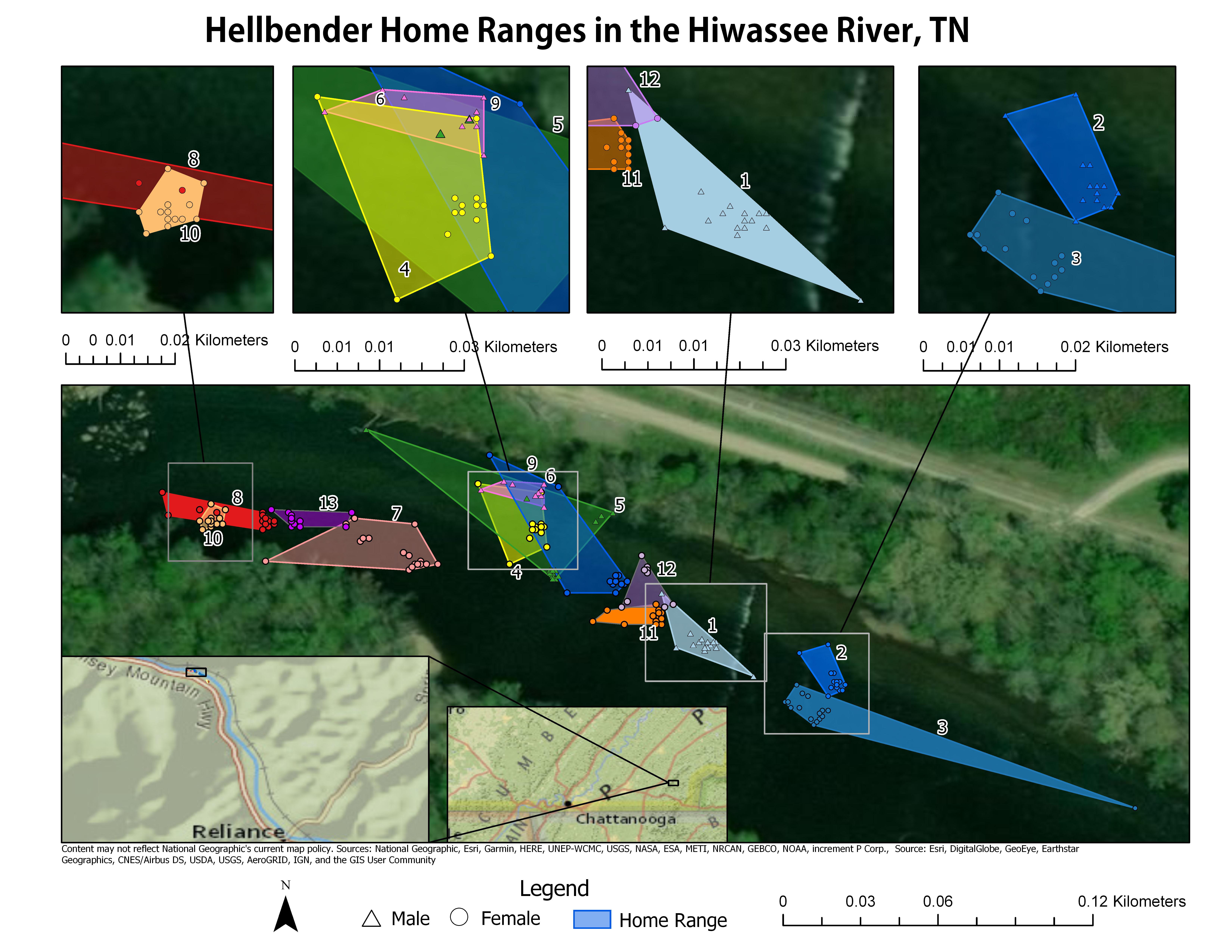
Meanwhile, when I’m not freezing out in the field – I’ll spend the rest of my time over the winter break reading over more literature about analyzing animal movements, a subject that volumes of articles have been written about. For now, I have been playing around with using kernel densities in Arc GIS Pro to analyze core home range sizes. This approach tells more about where the animals chose to spend the majority of their time. Unlike minimum convex polygons, which simply outline the entire extent that an animal may use – kernel densities focus on highlighting areas that are most important to the animal. 

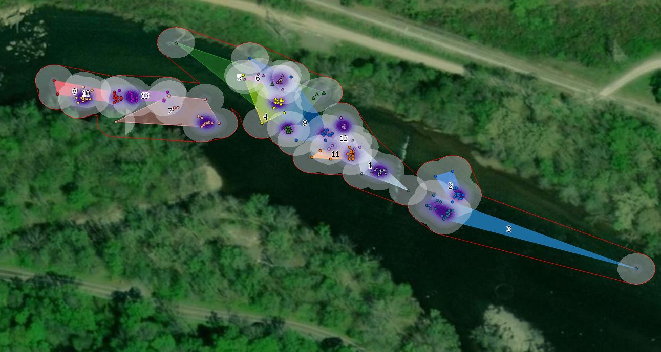
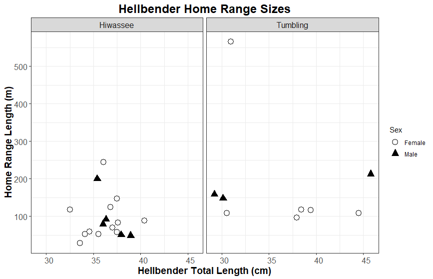
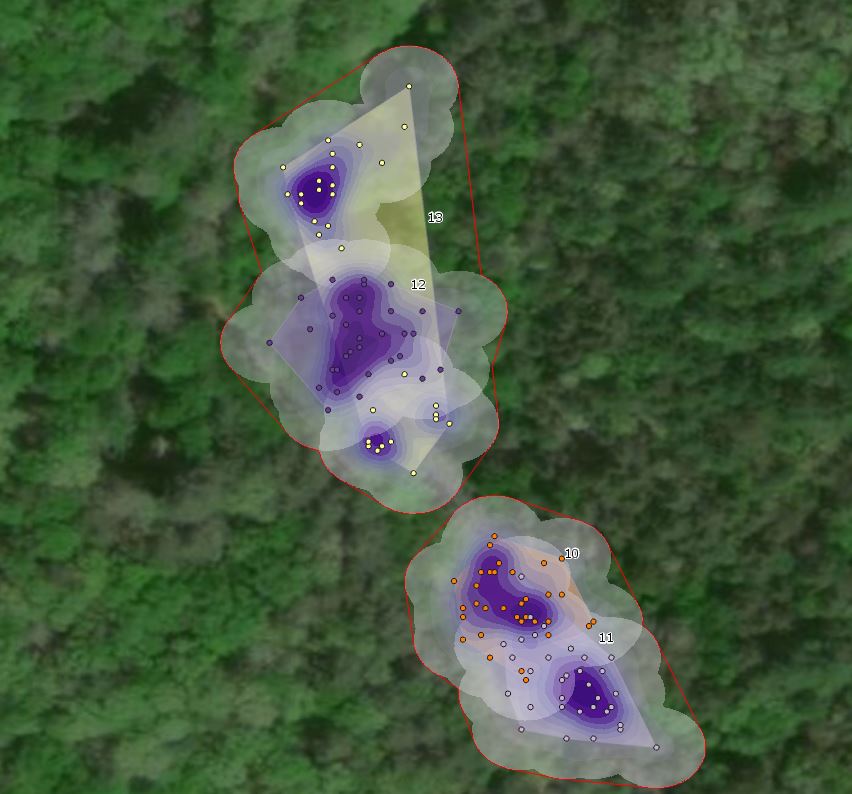
So far, our findings seem toindicate that when using kernel densities to determine the home ranges of thehellbenders, they have a very limited area that they tend to utilize most ofthe time. This makes sense, since hellbenders are largely sedentary throughoutthe year (with mating season in the fall being an exception). I haven’t had the chance to compare too many differences between Tumbling and Hiwassee – but upon first inspection it appears the home ranges in Tumbling are slightly larger than in Hiwassee. This fits with the amount of movement we saw in the Tumbling animals compared to those at Hiwassee, which often times were under the same rocks. This photo below shows an example of some kernel density home ranges in Tumbling creek. It is interesting to see how kernel densities can highlight the fact that while home ranges may appear overlapping with minimum convex polygons (e.g. 12 & 13), in reality when looking at the spatial use with kernel density analysis we see that 13 has used an area upstream and downstream of 12’s home range – but they did not generally overlap. 

By the time the spring rolls around, I hope to have done a fair bit of analysis on my data – so that it can be useful for predicting where to release our hellbenders for the best results. Furthermore, the data collected from these two streams will help us to compare the results from our translocation in order to understand the level of “success”. Granted, this is relative – since we are only able to track these animals for 2 years before the transmitters die. After that, we hope that the translocated individuals will reproduce and start to increase the populations in the streams where we are releasing them. Only time will tell! Stay tuned for more updates as the seasons change yet again. Until then, stay warm! 

The temperatures are beginning to drop here in Tennessee, and that means leaves are changing colors, school is in full swing, and the Hellbenders are entering their breeding season. We have been tracking our Hellbenders for about 4 months now, and we’ve seen some exciting developments in the past few weeks as they enter their breeding season. In order to fully appreciate what we have found, it helps to know a little bit about Hellbender reproduction.

Hellbenders are unique among amphibians, as the males are actually responsible for providing parental care to their offspring as they develop within their eggs. Male Hellbenders will seek out large flat rocks with plenty of space underneath and usually only one entrance that can easily be protected. They will fiercely defend this territory from other males, in the hopes of attracting a female to come lay her eggs there. Should they be so lucky, a female will lay a long string of hundreds of eggs, and the male will fertilize them externally. (Mayasich and Phillips, 2003). This means it is the females that generally wander around and look for a mate when the fall comes around.

At our Tumbling Creek location, we have one female that seems to be on a mission – she has moved almost 2 miles upstream, crossing the state line from Tennessee into Georgia! Could this be for breeding purposes? We aren’t sure. This past week in the field we re-captured her and took skin swabs from her to analyze the microbiome on her skin and also to check for diseases. This allowed us to get a good look at her for the first time in months, and she appears very healthy! Since we had to do surgery on the Hellbenders to input the transmitters, one thing we are checking when we re-capture animals is to see how their surgery wound is healing up. In the case of this individual, her wound was hardly noticeable – which is a great sign.

At our other location, the Hiwassee River, we also had some interesting developments. One of our animals there has been MIA for the past two weeks. We couldn’t get a signal in any direction upstream or downstream from where it was last located. The receiver has a range of about 100 meters, but the stream is large and it is entirely possible that the animal moved further than that – especially considering the sustained large moves made by the female on Tumbling Creek. This week however, we re-located that animal to exactly the same rock where it was last found before it went missing! Could it have gone off to breed and then returned “home” ? Quite possibly.

Unfortunately, we tracked a different animal at the Hiwassee to an unfortunate spot – the river bank. This almost certainly means the animal was subject to predation from otters, which we have seen from time to time there. Hellbenders do not have many predators, especially as adults – given their secretive lifestyle hiding under large boulders in streams, but with breeding season in action they are more prone to move around and therefore may have caught the eye of a hungry otter. 😦

The rest of our individuals have been so far not moved too far from their normal rocks – with a few exceptions of course. We head out again this weekend for one of the last field days of the season and I expect that we will find even more animals moving from their normal locations to breed before the weather turns colder. We re-captured another one of our animals on the Hiwassee, again to swab for the skin microbiome and diseases, and luckily it too seemed to be doing great. I will report back with more updates soon!

Welcome! My name is Brad and I’m a new Master’s Student at Tennessee State University studying the spatial ecology of Eastern Hellbenders in Dr. William Sutton’s Wildlife Ecology lab.  What is a Hellbender? What’s spatial ecology? Why bother to study that? – Good questions!

Hellbenders are the largest salamanders in North America; they can grow to be 2 feet long (~60 cm) and they can live for over 30 years (Taber et al. 1975). They’re fully aquatic, which means they spend their entire lives underwater – from egg to adult. They breathe through folds in their skin, which is also known as cutaneous respiration. These folds have earned them the nickname,  “ol’ lasagna sides.” They’re really cool animals! Most people never get to see one because they spend most of their lives hiding under rocks in cool, fast-moving mountain streams throughout the east coast of the United States.

Because Hellbenders live in the water and breathe through their skin, they are extremely susceptible to pollutants and other environmental contaminants. They require high quality habitat (think clear, cold water) in order to thrive – which is why they are often considered “indicator species” , meaning their presence is a sign of a healthy ecosystem. Unfortunately, Hellbenders are declining throughout their range in the eastern U.S. and they are currently being considered for endangered status by the U.S. Fish and Wildlife Service.  Luckily, in East Tennessee we have a few streams that currently support a large number of Hellbenders, such as the Hiwassee River, and the populations there seem to be doing well  (Freake and DePearno, 2017).

There are other streams in Tennessee however where Hellbenders aren’t doing as well as they used to be years ago. What’s worse, the Tennessee Valley Authority (TVA) has built dams on many of these streams so Hellbenders from healthy populations are no longer able to disperse into these areas. So, we have proposed a conservation strategy to help increase the populations in those streams where Hellbender numbers are dropping – move a few from the streams where there are plenty! But, we can’t just go out and move a bunch and call it a day. We need to study what types of movements they make and what types of habitats (i.e. parts of the stream) they use, in order to understand what they will need when they are moved to the new streams. This is spatial ecology – understanding how an animal uses the space around it. By understanding the habits of these Hellbenders, we will have a better idea of what is considered “normal” for them, essentially establishing a baseline. After the animals are moved – we will compare their movements in these new habitats to the baseline and see if this is a conservation strategy that works.

So how do we study the movements of these underwater salamanders? We use radio-telemetry – which involves a radio transmitter that is surgically implanted into the Hellbenders (we are currently tracking 25) and a receiver with an antennae that can pick up the signal from that transmitter. It sounds like a small “beep… beep…. beep,” and when you get closer to the animal, it will get louder. It is essentially a game of “hotter, colder” – and at the end you will find yourself standing over a rock, which presumably has a Hellbender hiding underneath it. Once we locate where they are hiding, we will take down some data about how big the rock is and how many other big rocks are nearby, along with a GPS point and other data that we believe may be important such as water temperature and flow rate.

Stay tuned to find out more about our adventures in the field and how the Hellbenders are doing!

Thanks for joining me!

Good company in a journey makes the way seem shorter. — Izaak Walton